38 Excel Formulas Every SEO Must Know

Table of Content

PPC SEO

Click to hear an audio recording of this post

Regarding using spreadsheets for tasks, the users’ loyalty is almost equally divided between Google Sheets and Microsoft Excel.

We have already covered the Google Sheet Formulas for SEO in one of our previous posts.
Well, then, why leave behind SEOs who prefer using Microsoft Excel over Google Sheets?

If you’re someone who loves Excel for organising and optimising your SEO workflows, this post is definitely for you!

We’ve discussed some of the most useful Excel for SEO formulas and their applications that can save a ton of time and make handling high-level SEO tasks easier than ever.

Let’s begin.

MS Excel Formulas for High-Level SEO Tasks

Although most of the formulas are the same in Google Sheets and Excel, their syntax and processes may vary.

That said, here’s the list of Excel formulas for SEO.

1. TEXT FUNCTIONS

The TEXT function in Excel allows you to format numbers, times, or dates as text in a specific format.

LEN

When you use the LEN formula on a text string, it returns the number of characters in that string.

Syntax: =LEN(text)

SEO use cases:

Analysing the length of meta descriptions and title tags

Evaluating PPC and ad copies

Identifying URLs that are too long, etc.

Example:

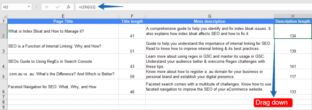
Let’s say we want to check the length of multiple titles and meta descriptions. As shown in the below screenshot we applied the formula in cells F2 & H2 and simply dragged it down.

And we have the number of characters for each of the titles and meta descriptions.

FIND

The FIND formula locates the position of a specified character or substring within a text string.

Syntax: =FIND(find_text,within_text,start_num)

SEO use cases:

Locating the position of a delimiter or query string (“?” in URLs).

Identifying the start position of campaign parameters for data extraction.

Analysing keyword placement within a URL for better URL optimisation

Example:

Let’s say we want to find the position of the question mark in a URL (to locate where the query parameters begin).

We have all the URLs in column A. Applying the formula =FIND(“?”, A2) in column B will return the position of the “?” in each URL.

Then, we need to drag the formula down to find the positions for other URLs in the list, as shared in the screenshot below.

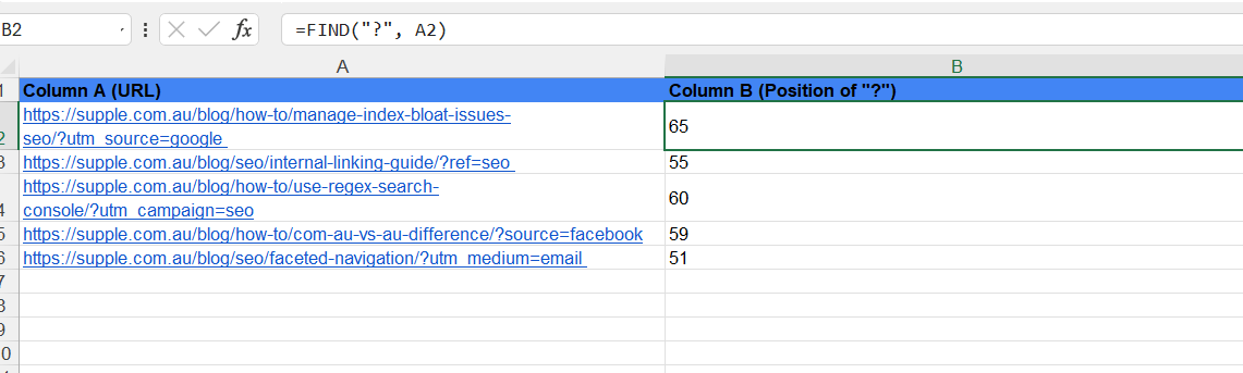
Image Note: we need to show one arrow at the formula and one drag-down arrow at “65.” (B2) Check the reference image.

LEFT

The LEFT formula lets you pull out a specific number of characters from the start of a text string.

Syntax: =LEFT(text,num_chars)

SEO use cases:

Extracting primary keywords or prefixes from long-tail keywords.
Analysing category tags or prefixes in URL structures

Example:

Say we download a competitor’s backlink report. We need to clean up the URLs by extracting only the domain, which is perfect for outreach or domain analysis.

So, we use the following formula rather than manually editing each URL.

=LEFT(C2, FIND(“/”, C2, FIND(“//”, C2) + 2))

It first finds the position of “//” to skip over the protocol (http:// or https://), then looks for the first “/” after the protocol to identify the end of the domain.

Finally, it uses the LEFT function to pull out everything from the start of the URL up to “/,” returning the base domain.

This gives us the domain from column C. Next, we drag the formula down column D, as shown in the attached screenshot. It automatically applies to all rows and gives clean URLs.

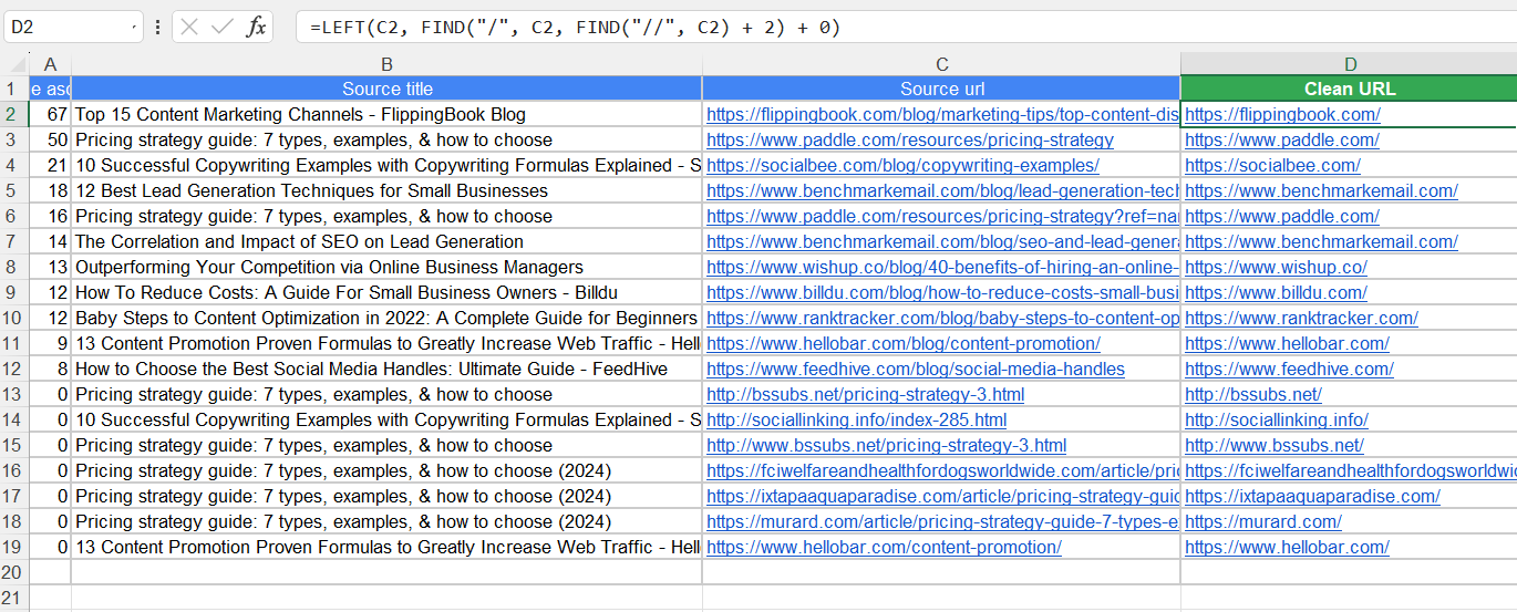
Image Note: We need to display an arrow pointing at the formula and another pointing down at the clean URL in cell D2. Here’s a ref image -

RIGHT

The RIGHT formula helps you extract a specified number of characters starting from the end of a text string.

Syntax: =RIGHT(text,num_chars)

SEO use cases:

Extracting file extensions from URL paths (.html, .xml).
Identifying campaign tags at the end of UTM parameters in URLs.

Example:

Let’s say we download an indexed pages report from Google Search Console to analyse indexed URLs and identify different URIs pointing to the same content.

So, we use the following formula to extract just the URI from each URL.

=RIGHT(A2, LEN(A2) - FIND(“/”, A2, FIND(“//”, A2) + 2))

The formula works by first finding the total length of the URL using LEN(A2). It then locates the position of the first “/” after the domain by using FIND(“/”, A2, FIND(“//”, A2) + 2). This helps to identify where the domain ends and the URI begins. By subtracting the position of this ”/” from the total length, it calculates how much of the URL to keep. The RIGHT function then takes that part of the URL, which is the URI.

Next, we drag the formula down column C, applying it to all rows automatically, as shown in the screenshot below. This allows us to identify inconsistent URIs.

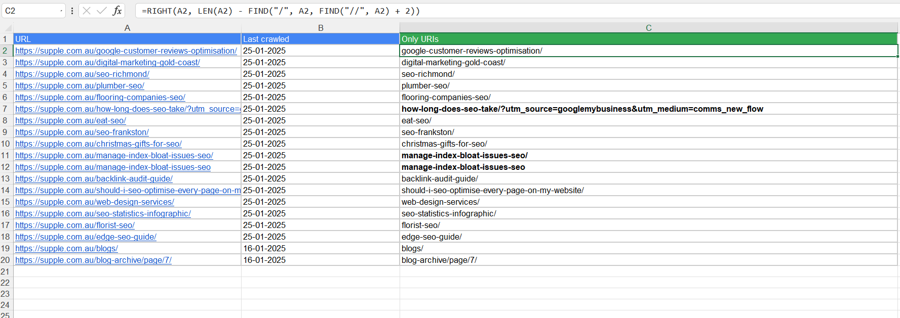
Image Note: we need to show one arrow at the formula and one drag-down arrow at C2.

Check the reference image shared above.

MID

The MID formula lets you pull out a specific number of characters from a text string, starting exactly where you want and continuing for as many characters as you specify.

Syntax: =MID(text, start_num, num_chars)

SEO use cases:

Extracting keywords or slugs from URLs.
Extracting campaign parameters from URLs.

Example:

Assume we’ve downloaded a combined NAP (Name, Address, Phone Number) dataset for Local SEO Citations Management or Google Business Profile Audits for our local SEO clients.

Now, we need to extract the Name, Address, and Phone Number from this combined data set.

So, we apply the formula: =MID(A2, FIND(“|”, A2) + 2, FIND(“|”, A2, FIND(“|”, A2) + 2) - FIND(“|”, A2) - 2)

The MID function then extracts everything between these two positions. This helps us extract the address from column A into column C.

Next, we drag the formula down column C to automatically apply it to all rows, extracting the Address for each entry, as shown below.

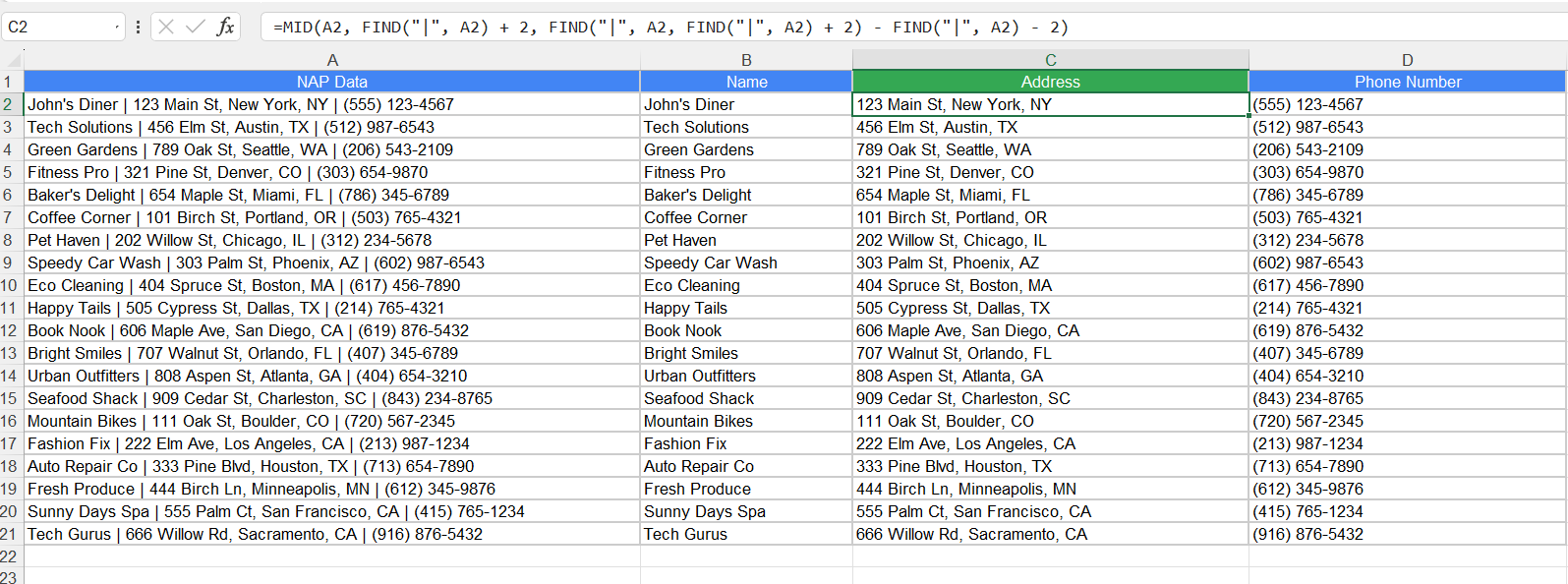
Image Note: We need to show one arrow at the formula and one drag-down arrow at C2.

UPPER/LOWER/PROPER

The UPPER LOWER PROPER formulas allow you to change the case of selected text or data sets into uppercase, lowercase, and proper case (title case).

Syntax:

=UPPER(text)

=LOWER(text)

=PROPER(text)

SEO use cases:

Keeping consistency in the title tags format
Keeping the consistency in meta descriptions format

Capitalising acronyms, etc.

Example:

Here, we have all the page titles in lowercase format. However, we want to change them into a title case. Therefore, we added =PROPER(A2) in B2 and dragged it down.

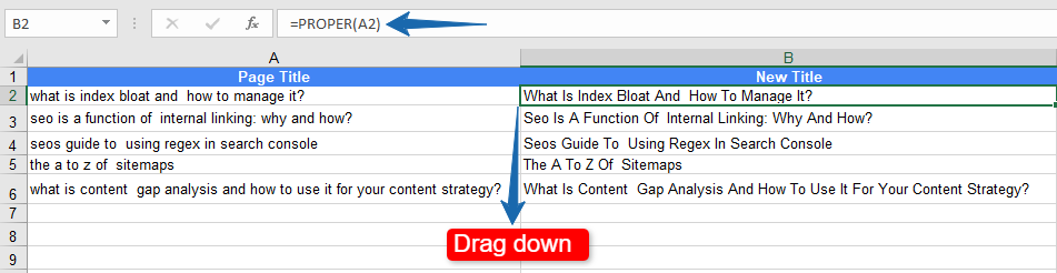
And there you have it. The text is converted in the proper case.

EXACT

The EXACT function lets you compare two text strings and marks the corresponding cell as TRUE if they are exactly the same. Otherwise, it’ll mark the cell as FALSE.

Syntax: EXACT(text1, text2)

SEO use cases:

Matching keywords data — especially long-tail keywords
Compare titles, meta descriptions, URLs, etc.

Example:

Here, we have the list of titles in Columns D and F and we want to check if they’re exactly the same. Hence, we entered the formula =EXACT(D2, F2) in G2.

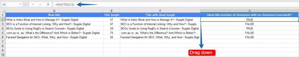
The titles that are an exact match are marked TRUE, and FALSE otherwise.

Similarly, you can compare comprehensive lists of long-tail keywords or meta descriptions.

TEXT TO COLUMNS

Text to Columns function helps you split the data of one cell/column into multiple cells/columns.

Syntax: Text to Columns is not a formula, it’s a process.

SEO use cases:

Breaking up URLs into multiple parts such as protocol, domain, path, parameters, fragments, etc.

Splitting full names into first and last names
Breaking up comma-separated values (CSVs) into separate columns, etc.

Example:

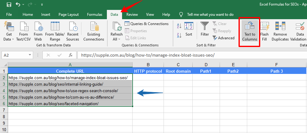
We have a list of URLs and we want to break them down into separate columns named according to the parts of the URL.

For this, we selected the URLs and clicked Data. Then we selected the Text to Columns function from the menu as shown below.

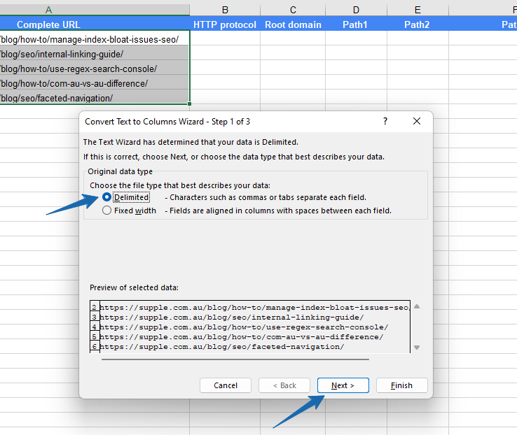
On the next screen, we clicked Delimited and hit Next.

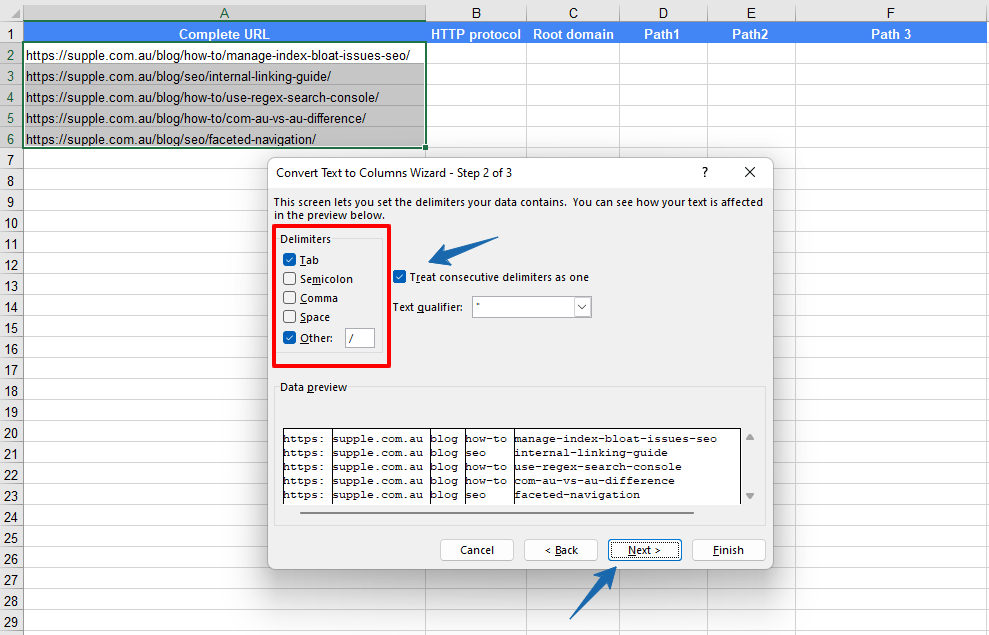
Here, we entered Trailing Slash (/) as the delimiter and allowed to “Treat consecutive delimiters as one” and clicked Next.

Next, we had to choose the destination where we wanted to place the data. So we clicked the cell B2 and hit Finish.

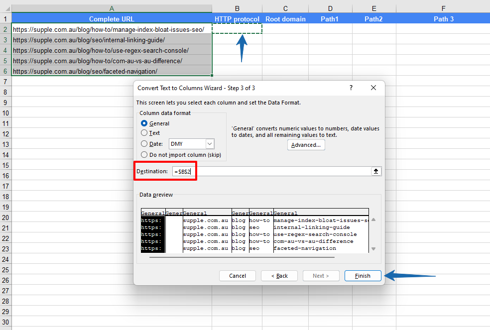
And there you go.

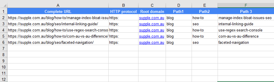
The URLs are broken down into relevant parts corresponding to the column titles.

2. LOOKUP FUNCTIONS

Lookup functions in Excel allow you to search for a value in a range or table and return a related value from a different column or row.

VLOOKUP

VLOOKUP helps you pull the data from one Excel sheet to another by using a formula instead of copying and pasting them manually.

Syntax: VLOOKUP (lookup_value, table_array, col_index_num, [range_lookup])

SEO use cases:

Pulling or sharing keyword data between different sheets
Combining different datasets to make a master sheet

Combining data from multiple sheets for SEO/Content/Backlink audit, etc.

Example:

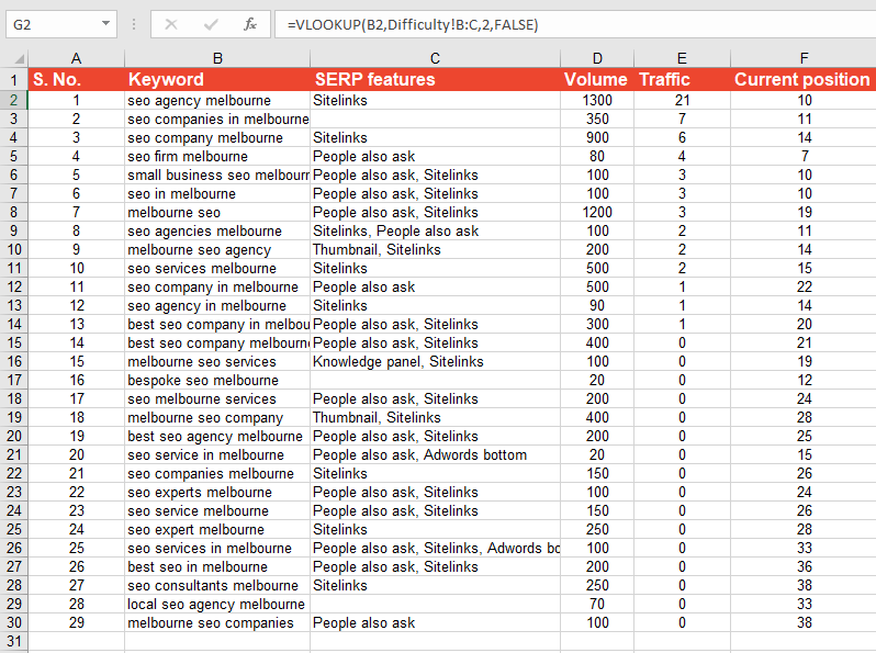
Let’s say we have a set of SEO data such as keywords, SERP features, volume, traffic, etc. in one sheet. We’ll call it Sheet 1 and it looks like this.

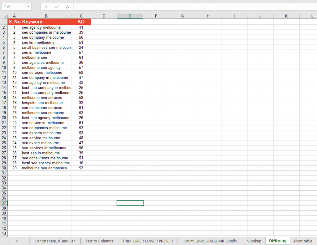
And there’s Sheet 2 that holds the keyword difficulty (KD) score for the keywords mentioned in Sheet 1. It looks like this.

Now we want to pull the KD score in Sheet 1. So we used this formula in G2: =VLOOKUP(B2,Difficulty!B:C,2,FALSE)

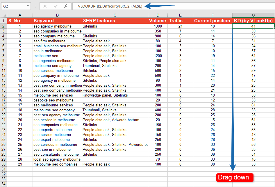
Then we simply dragged it down from G2 to G30.

And there it is. All the KD score data is right there in Sheet 1.

As an SEO, you might be creating multiple Excel sheets for different types of data and sometimes you might need to combine multiple sheets. That’s where VLOOKUP can save you time that goes into copying and pasting time and again.

Besides, the data in the master sheet gets updated automatically when you change values in source sheets.

XLOOKUP

XLOOKUP allows you to quickly find specific data based on a search criterion. This can be helpful for SEO tasks like looking up keyword rankings or search volumes. It can help search for exact matches or approximate ones and even handle multiple criteria for more complex searches.

Syntax: =XLOOKUP(lookup_value, lookup_array, return_array, [if_not_found], [match_mode], [search_mode])

SEO use cases:

Find keyword rankings based on search terms for targeted optimisation.
Retrieve historical organic traffic data for better content performance analysis.

Example:

Suppose we have a list of keywords and their corresponding difficulty scores. If we want to find the keyword difficulty for “Google trends,” we can use the formula:

=XLOOKUP(E2,A2:A12,D2:D12)

This looks for “Google trends” in column A (keyword list) and returns the corresponding keyword difficulty from column D.

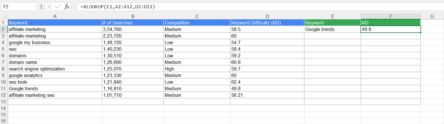
Image note: we need to show one arrow at the formula AND ONE AT 49.8.

INDEX

The INDEX formula allows you to retrieve a value from a specific position in a given range or array. It’s helpful when you want to return a value based on its row and column numbers.

Syntax: INDEX(array, row_num, [column_num])

SEO use cases:

Pulling values from large datasets where you know the row and column but don’t need a full lookup.
Creating dynamic reports that pull specific values based on changing criteria, like keywords and traffic.
Pulling values from keyword or traffic data within large, organised datasets for SEO performance reports.

Example:

Let’s say we have a dataset where column A contains search volumes and column B lists the associated keywords.

Now, we want to find the keyword with the highest search volume. So, we use the formula =INDEX(B2:B11, MATCH(MAX(A2:A11), A2:A11, 0)) in cell C2.

The MAX(A2:A11) part of the formula identifies the highest search volume, which is 1900 in this case. The MATCH(MAX(A2:A11), A2:A11, 0) function then finds the position of this maximum value within the search volume column.

Finally, the INDEX(B2:B11, MATCH(...)) function returns the corresponding keyword, which is “marketing operations” as shown in the screenshot below. This allows us to find the keyword with the highest search volume without hassles.

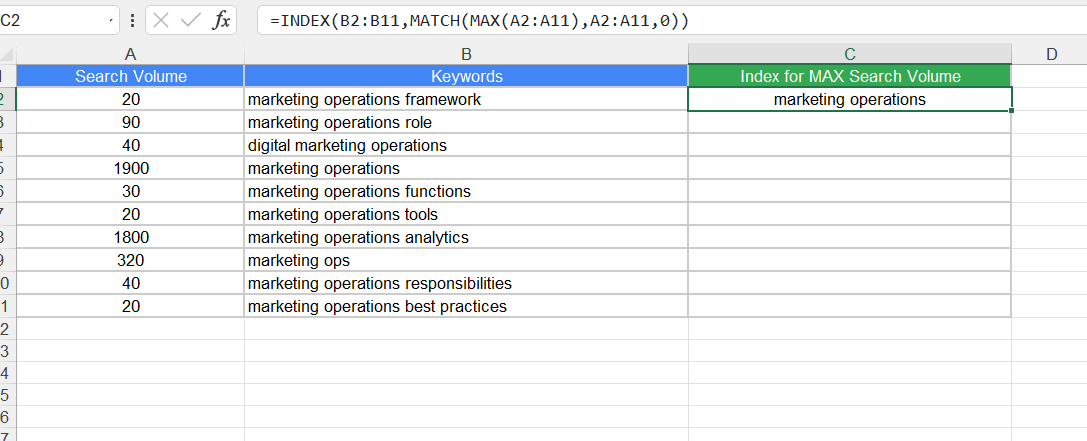
Image Note: One arrow should point at the formula and another at C2.

MATCH

The MATCH function lets you search for a value within a range or array and return its relative position. It’s often combined with functions like INDEX to create dynamic lookups.

Syntax: MATCH(lookup_value, lookup_array, [match_type])

SEO use cases:

Locating keyword position in a ranking list to track SEO performance.
Matching competitor URLs to identify ranking shifts
Finding the exact search volume based on keyword rank.

Example:

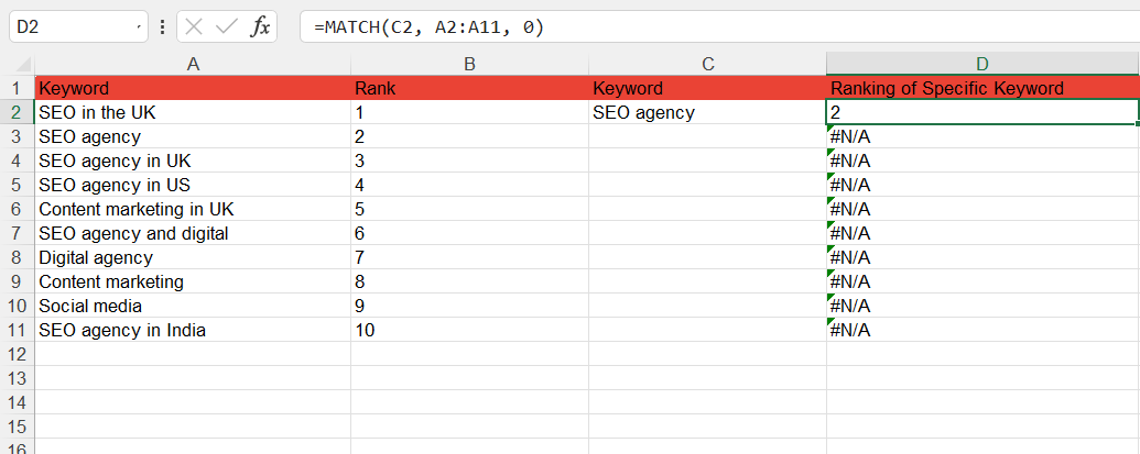
We have a list of keywords in column A and their rankings in column B. Here, we want to find the position of a specific keyword, “SEO agency” in the list.

So, we apply the formula =MATCH(D2, A2:A11, 0) and drag it down. It gives its ranking as 2 when it finds a match.

The rest of the rows show N/A as it doesn’t find any exact match. See the screenshot below to find the final output.

Note: One arrow should point at the formula and another at cell D2, showing the drag-down action.

3. CONDITIONAL FUNCTIONS

Conditional functions in Excel, like IF, COUNTIF, and SUMIF, help you perform actions based on certain conditions. They make it easy to analyse data by applying rules.

IF

IF function allows you to check whether a specific condition is met. And it returns the answer or value as you mention in syntax.

Syntax: IF(logical_test, value_if_true, [value_if_false])

SEO use cases:

Determining whether the URLs match
Checking if the keywords are worth targeting based on their search volumes
Marking the titles and meta descriptions’ character length as Yes/No or Good/Bad, etc.

Example:

In the above example, we calculated the length of meta descriptions. Now we want to check whether the length of meta descriptions is within the recommended range i.e. less than 160 characters.

Hence, we entered the formula =IF(H2<160, “Yes”,”No”) in the I2.

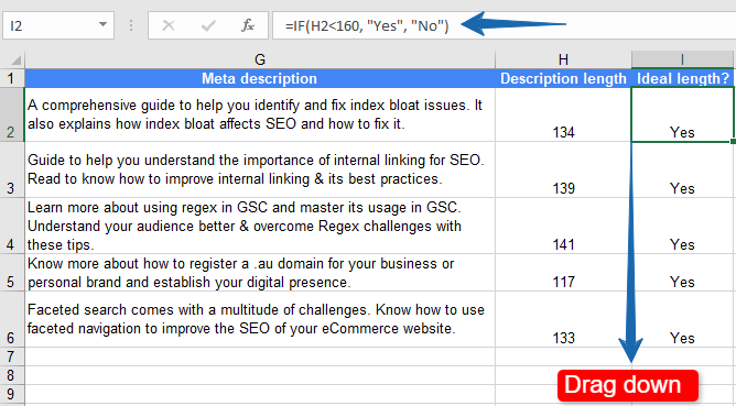
Since all the meta descriptions in this example meet the condition the corresponding cells are marked as Yes. Had any of them exceeded 160 characters in length, the cell next to it would’ve returned the value as No.

SEARCH with IF and IFERROR

In this example, we’ll show how you can combine different formulas and manipulate your SEO datasets. Let’s understand these formulas individually first.

SEARCH: Returns the position of a substring within a string
IF: Marks the cells as YES or NO based on whether the condition matched or not

IFERROR: Returns the value that you specify in case the formula returns an error

Syntax:

SEARCH(find_text,within_text,[start_num])

IF(logical_test, value_if_true, [value_if_false])

IFERROR(value,value_if_error)

SEO use cases:

Sorting keywords
Grouping URLs
Grouping content assets based on their types, categories, taxonomy, etc.

Example:

We have a list of URLs for different types of content resources. Now, we want to identify and sort them according to their types.

So we name columns B, C, and D as Guide, Tool, and Blog Post respectively. Next, we applied these formulas:

Cell B2: =IFERROR(IF(SEARCH(“/guides”,A2),”Yes”,”No”),”No”)

Cell C2: =IFERROR(IF(SEARCH(“/tools”,A2),”Yes”,”No”),”No”)

Cell D2: =IFERROR(IF(SEARCH(“/blog”,A2),”Yes”,”No”),”No”)

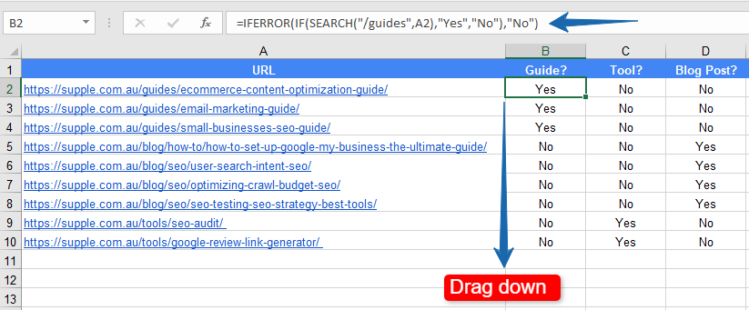
Thus, wherever the conditions match the cells are populated with “Yes”. And where they didn’t match or returned errors, the cells are marked “No”.

COUNTIF

The COUNTIF formula gives you the count of cells with specific attributes as entered by you while typing the syntax.

Syntax: COUNTIF(range, criteria)

SEO use cases:

Knowing the count of keywords with a certain search volume or ranking difficulty
Getting the count of URLs according to their categories
Knowing the count of duplicate keywords or URLs, etc.

Example:

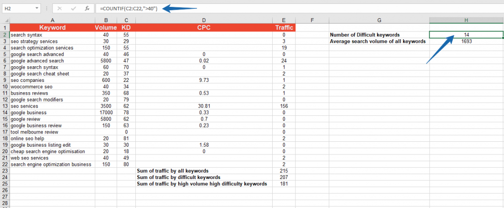
For instance, here we’ve applied the formula =COUNTIF(C2:C22,”>40”) in H2. It means counting the number of cells with a keyword difficulty (KD) score of more than 40.

There are 14 such keywords.

Thus, you can filter out the keywords with a specific difficulty score and decide whether to target them or not.

SUMIF

The SUMIF formula helps you add the numeric values from different cells that meet specific criteria.

Syntax: SUMIF(range, criteria, [sum_range])

SEO use cases:

Calculating the total website traffic data based on specific criteria
Sorting and manipulating the datasets
Adding up the search volume of keywords with high or low difficulty, etc.

Example:

Now, we want to calculate the total traffic for the keywords with a difficulty score above 40. Here’s the formula we used in cell E24: =sumif(C2:C22,”>40”, E2:E22).

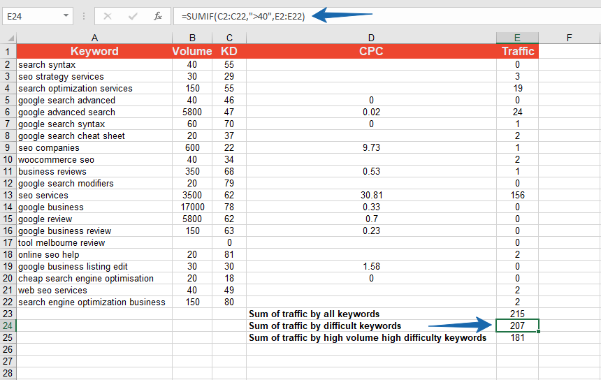
This function can be useful for understanding the difference in traffic generated from high and low-difficulty keywords. Accordingly, you can finetune your keyword strategy.

Also, if you’re not sure how to create the right keyword strategy for your business, you can hire external SEO services for the same.

4. ARRAY FORMULAS

Array formulas allow you to perform multiple calculations on one or more items in an array, returning a single result or multiple results. They are helpful for complex calculations and data analysis tasks.

ARRAYFORMULA

This function allows you to do calculations on an entire range of data without copying the formula down to each cell. It processes multiple rows at once.

Syntax: =ARRAYFORMULA(array_formula)

SEO use cases:

Applying formulas across entire columns or rows without dragging the formula down.
Automatically generating values like keyword lengths or rankings for large datasets.
Speeding up bulk SEO tasks, such as calculating traffic per keyword.

Example:

Let’s say we want to calculate the length of each keyword in a list to check if they’re within SEO-friendly character limits.

Here, we use an ARRAY FORMULA to process the entire range rather than applying the formula to each cell.

We will write the formula =ARRAYFORMULA(LEN(A2:A15)) in B2 and drag it down. This automatically counts all characters, including spaces, and returns the length for each keyword in the range.

For instance, in the below-shared screenshot, the keyword “seo agency melbourne” has 20 characters (15 letters + 3 spaces + 2 words), while “best seo companies” has 18 characters (16 letters + 2 spaces).

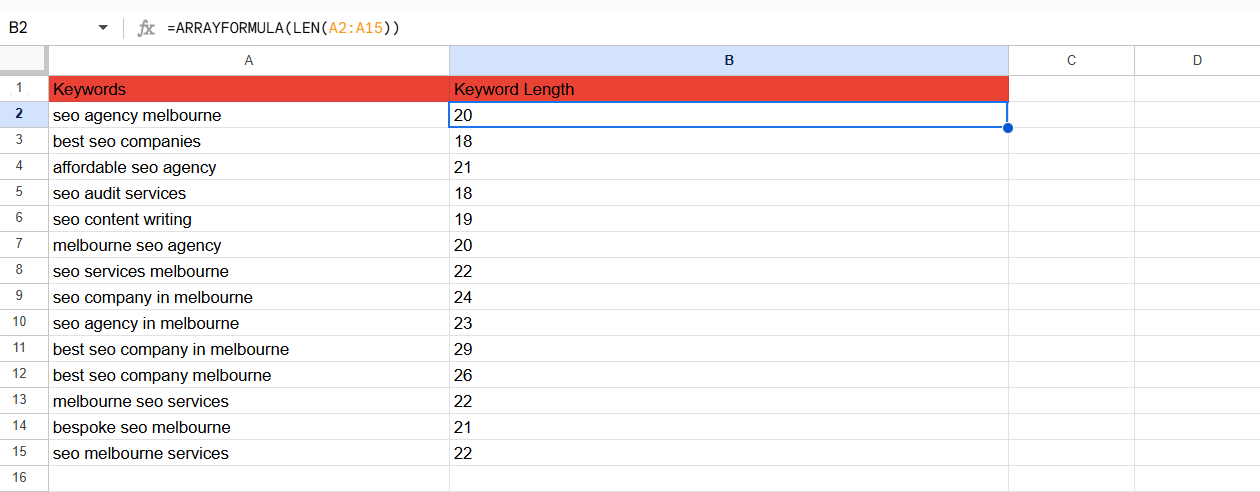
Image Note: We need to show one arrow at the formula and one drag-down arrow at “20” (B2).

TRANSPOSE

This function allows you to switch rows into columns or columns into rows in Excel or Google Sheets.

Syntax: =TRANSPOSE(array)

SEO use cases:

Reformatting keyword lists to fit specific tools or templates.
Converting vertical keyword data into a horizontal layout for reports.
Simplifying the structure of datasets for better analysis.

Example:

Say we have a list of page URLs and their corresponding hreflang values stacked vertically. This makes it difficult to compare and analyse the hreflang implementation across pages.

So, we use the formula: =TRANSPOSE(A2:A45) to convert those vertical hreflang values into a horizontal row. This approach makes it easy to analyse the implementation, as shown in the screenshot below.

This allows us to quickly compare the hreflang values for each page and identify missing or incorrect values.

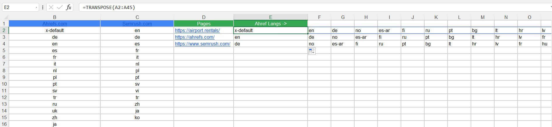
Image Note: One arrow at the formula and another horizontal arrow across the hreflang values

UNIQUE

The =UNIQUE formula helps you extract distinct values from a dataset by removing duplicates. This is particularly useful for cleaning and organising SEO data.

Syntax: =UNIQUE(range)

SEO use cases:

Deduplicating keyword lists to avoid redundant targeting.
Extracting unique domains from a list of URLs.
Identifying unique values in datasets for better analysis.

Example:

Let’s say we have a list of keywords, and some of them are repeated.

We want to extract only the unique keywords to avoid duplicate targeting in our SEO strategy. So, we can use the UNIQUE formula rather than manually sorting through the list.

Entering =UNIQUE(A2:A20) in cell B2, we process the range A2:A20 to extract distinct keywords and remove duplicates. The output dynamically updates if we make any changes to the input data.

The repeated keywords in column A are filtered into a unique list in column B, as shown in the attached screenshot. This approach makes it easy to streamline our SEO strategy.

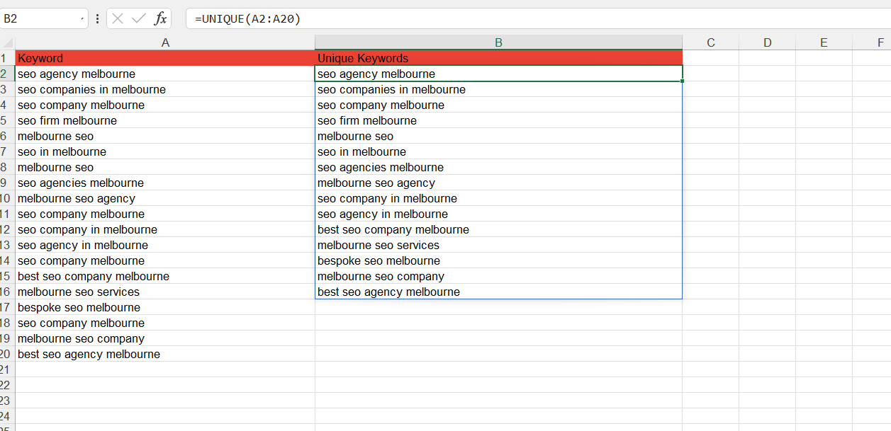
Image Note: We need to show one arrow at the formula and one drag-down arrow at “seo agency melbourne” (B2).

5. STRING SEARCHING and REPLACEMENT

String searching and replacement in Excel involve locating specific text within cells and replacing it with new text. This is helpful for tasks like reformatting URLs, fixing typos, or updating keywords in bulk.

SEARCH

The =SEARCH formula allows you to find the position of a specific substring within a text string. It’s case-insensitive, making it handy for analysing SEO data.

Syntax: =SEARCH(find_text, within_text, [start_num])

SEO use cases:

Finding specific keywords in meta descriptions or title tags.
Identifying the presence of branded terms within URLs.
Analysing text strings to locate crucial substrings.

Example:

Let’s say we have a list of meta descriptions, and we want to find the position of the keyword “SEO” in each description.

Now, we enter the formula =SEARCH(“SEO”, A2) in cell B2, as shown in the screenshot.

The formula looks for the word “SEO” in each description in column A and returns its position. If “SEO” is found, the formula gives its position. For instance, see the screenshot. It shows 113 for the first row.

On the other hand, if “SEO” is not found, it returns “#VALUE!” as shown in the attached screenshot. This helps us identify where the keyword appears in each meta description.

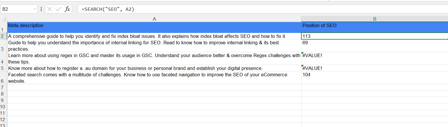
Image Note: we need to show one arrow at the formula and one drag-down arrow at “113” (B2)

SUBSTITUTE

With the SUBSTITUTE formula, you can replace any character or word with another word.

Syntax: SUBSTITUTE(text, old_text, new_text, [instance_num])

SEO use cases:

Editing on-page SEO elements like title tags or meta descriptions at scale
Updating the URLs or parts of the URLs quickly
Changing or redirecting the URLs during the website migration process, etc.

Example:

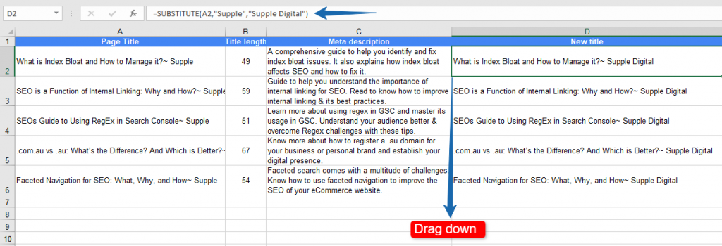
Refer to Column A in the screenshot below. We want to replace “Supple” with “Supple Digital” at the end of the titles. We did this by inserting the =SUBSTITUTE(A2,”Supple”,”Supple Digital”) formula in D2.

Thus, you can edit titles, URLs, and meta descriptions at scale with this function.

TRIM

When you apply the TRIM formula, it removes the extra blank spaces from text or string.

Syntax: =TRIM(text)

SEO use cases:

Removing extra spaces in data exported from SEO tools
Removing extra spaces in data copied from a different file format, etc.

Example:

Take a look at the titles in Column B. As highlighted, there are extra spaces in each of them. And we could remove them by using the =TRIM(B2) formula in cell C2.

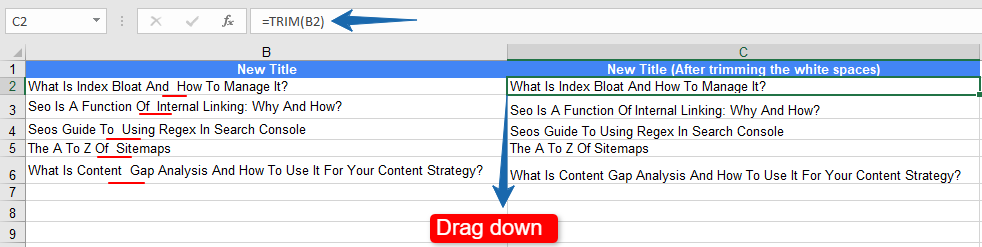
For a sample size this small, it’s easy to remove extra spaces manually. But for huge datasets, it’s not feasible.

Besides, a single extra space here and there is difficult to locate when you’re dealing with hundreds of titles. That’s where you can keep your title consistent with this formula.

CLEAN

This function helps you remove all non-printable characters from a text string. It helps clean messy data imported from other sources, such as scraped content or exported reports.

Syntax: =CLEAN(text)

SEO use cases:

Cleaning keyword lists with hidden non-printable characters.
Preparing content scraped from the web for analysis.

Example:

We have a list of keywords with unwanted non-printable characters that may interfere with SEO tools or analysis.

So, we use the formula =CLEAN(A2) in B2. The formula processes the keywords in column A, removing non-printable characters like line breaks, tabs, and non-breaking spaces.

This gives us cleaned keywords ready for analysis or for importing into SEO tools, as shown in the attached screenshot.

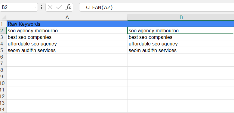
Image Note: We need to show one arrow at the formula and one drag-down arrow at “seo agency melbourne” (B2)

6. PIVOT TABLES WITH CALCULATED FIELDS

Pivot table lets you group data from different columns, extract trends from comprehensive datasets, and provide a table of summary.

Syntax: Since the pivot table is not a formula, it doesn’t have a syntax. Instead, it’s a step-by-step process that we’ve shared in the example.

SEO use cases:

Analysing the changes in ranking for different pages
Analysing traffic based on GA data
Reviewing site architecture using crawl data, etc.

Example:

Being an SEO agency, we also keep upgrading our SEO strategies regularly. Therefore, we want to extract certain trends from our keywords dataset and get a summary in a pivot table.

Here’s the keyword data and we want to generate a pivot table for the same. So we selected the data range and clicked Insert.

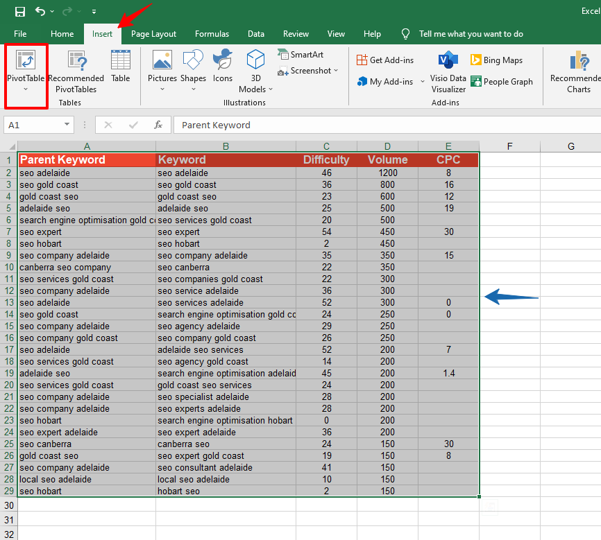
From the Insert menu, we selected Pivot Table.

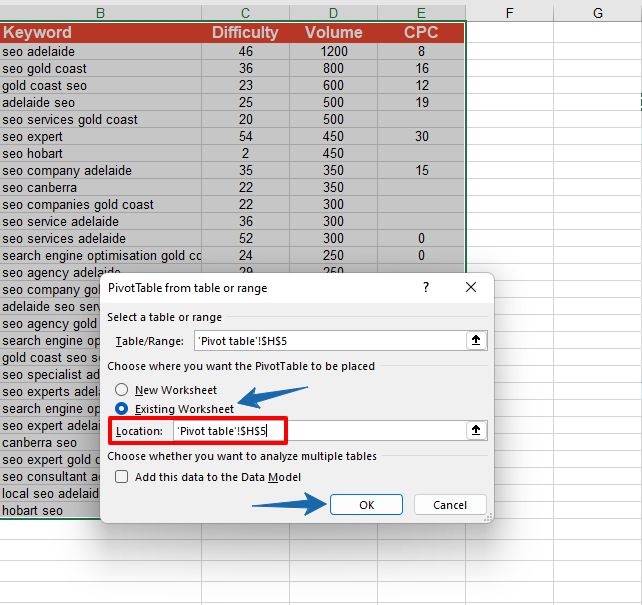
Next, we clicked Existing Worksheet since we wanted the pivot table on the same sheet. And clicked the cell H5 to select the location where we want to place the table and hit OK.

In the next screen, we select the fields that we want to include in the pivot table. For instance, we chose fields like Parent Keyword, Difficulty, and Volume.

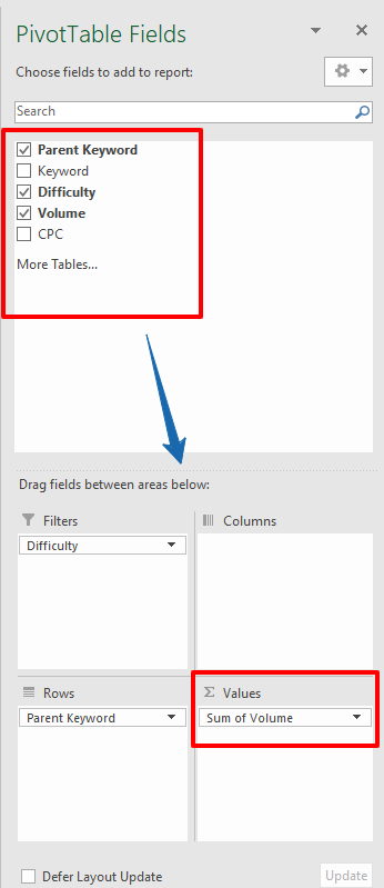
And clicked Sum of Volume to modify the settings for this field.

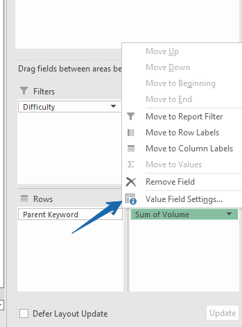
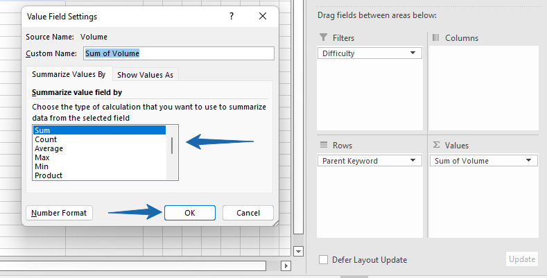
Here, you can select how you want to manipulate the data for this field. Since it’s for illustration purposes, we went ahead with the simple Sum function and clicked OK.

However, you can also do advanced calculations in pivot tables.

Here’s what the pivot table looks like.

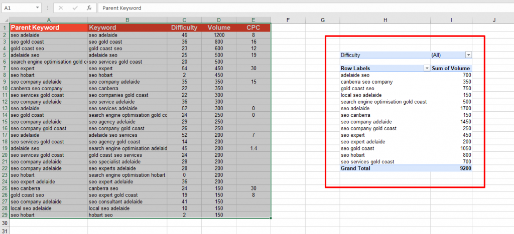
The pivot table has a list of unique parent keywords extracted from column A and the sum of the search volume for each of the keywords that belong to parent keywords. Also, we have a total of the search volumes.

This can help us identify the parent keyword that is more popular and we can thus keep that keyword as the focus keyword of the content/page we are planning to optimise for SEO.

7. DATE FUNCTIONS

Date functions in Excel allow you to work with and manipulate dates easily. They help calculate age, find differences between dates, or automatically display the current date in your worksheets.

TODAY

The =TODAY formula returns the current date dynamically. It updates automatically whenever the sheet is refreshed or reopened.

Syntax: =TODAY()

SEO use cases:

Tracking deadlines for SEO tasks or campaigns.
Calculating the age of content, like blog posts or URLs.
Creating daily reports with dynamic “date” updates.

Example:

Let’s say we want to calculate how old our blog posts are, based on their publication date, to decide if they need updates.

So, we enter the formula =TODAY() in C2, as shown in the screenshot below. Next, we apply it to the entire column by dragging down the formula. This ensures that each row shows the current date.

It displays the current date and updates dynamically every time the file is refreshed or reopened.

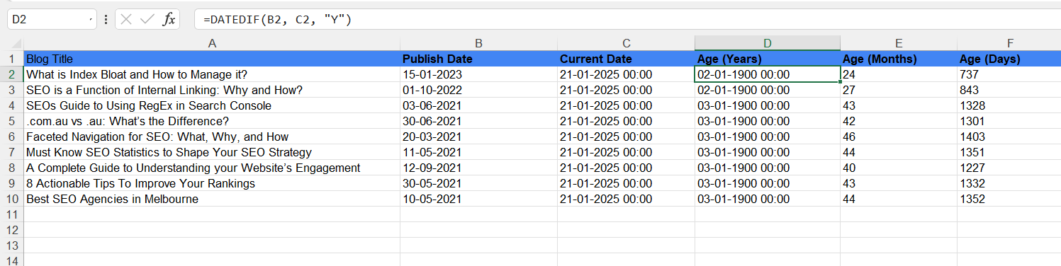
Image Note: One arrow should point at the formula, and another drag-down arrow should point at “current date 21-01-2025” in cell C2.

Next, we add =DATEDIF(B2, C2, “d”) in D2, which calculates the age of the content in days by finding the difference between the publication date in column B and today’s date in column C.

Next, we apply it to the rest of the rows by dragging the formula down. This helps calculate the age for each blog post.

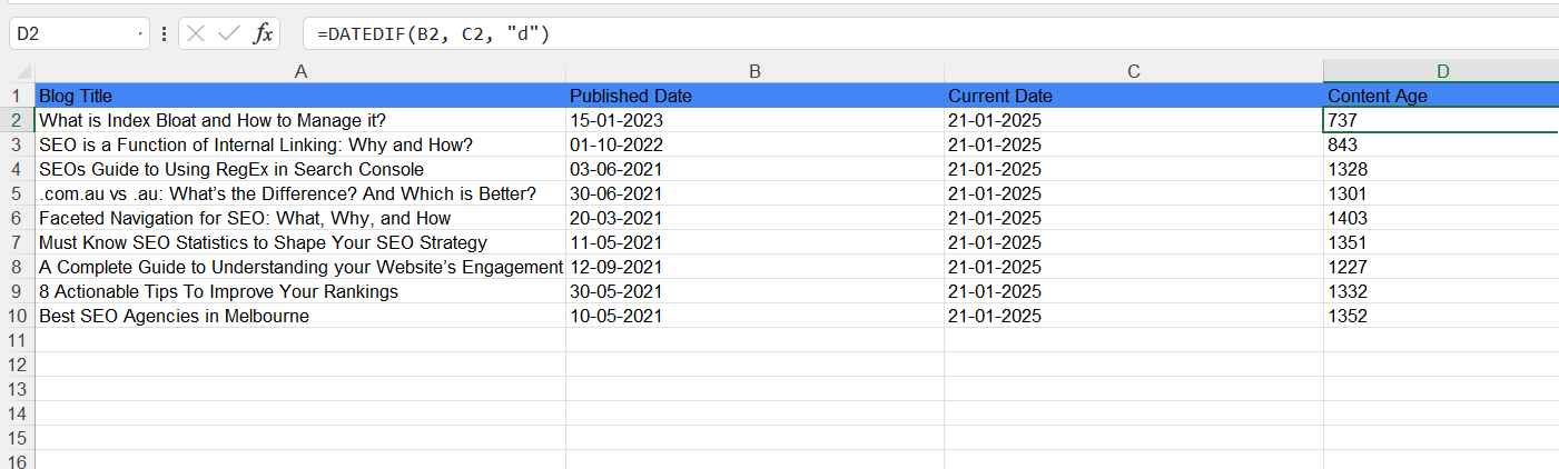
Image Note: One arrow should point at the formula, and another drag-down arrow should point at “current age 737” in cell D2.

NOW

The =NOW formula returns the current date and time, dynamically updating whenever the sheet is recalculated. It’s useful for time-sensitive SEO tasks, such as tracking deadlines, timestamps, or campaign schedules.

Syntax: =NOW()

SEO use cases:

Tracking timestamps for content publishing or updates.
Creating real-time reports with the current date and time.
Automating time-sensitive workflows in SEO campaigns.

Example:

Let’s say we’re managing a publishing schedule and want to track the exact time of updates.

We use the formula =NOW() in column C. It dynamically fetches the current date and time, as shared in the screenshot below.

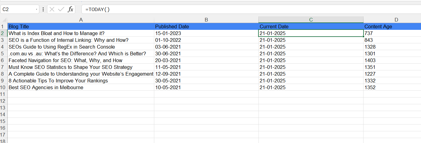
Image Note: One arrow should point at the formula, and another drag-down arrow should point at “C2 21-01-2025 19:56.”

Next, we enter =C$2 - B2 in column D, which subtracts the last update date in column B from the current time in column C. Notice the screenshot below to see the results.

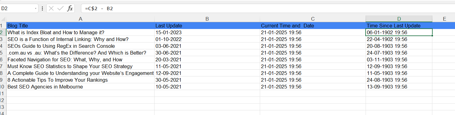
Image Note: One arrow should point at the formula, and another drag-down arrow should point at “Time since the last update” in cell D2.

DATEDIF

The =DATEDIF formula allows you to calculate the difference between two dates in terms of days, months, or years. It’s helpful for tasks where date intervals are crucial, such as tracking content age or SEO campaign durations.

Syntax: =DATEDIF(start_date, end_date, unit)

SEO use cases:

Tracking how old a blog post is for content refresh priorities.
Monitoring the duration of an SEO campaign.
Calculating time gaps between backlinks or updates.

Example:

Let’s say we want to calculate the age of our content in years, months, and days based on the publish date.

First, we use =TODAY() in column C, which automatically updates to today’s date. As shown in the screenshot, we drag the formula down to apply it to the rest of the rows.

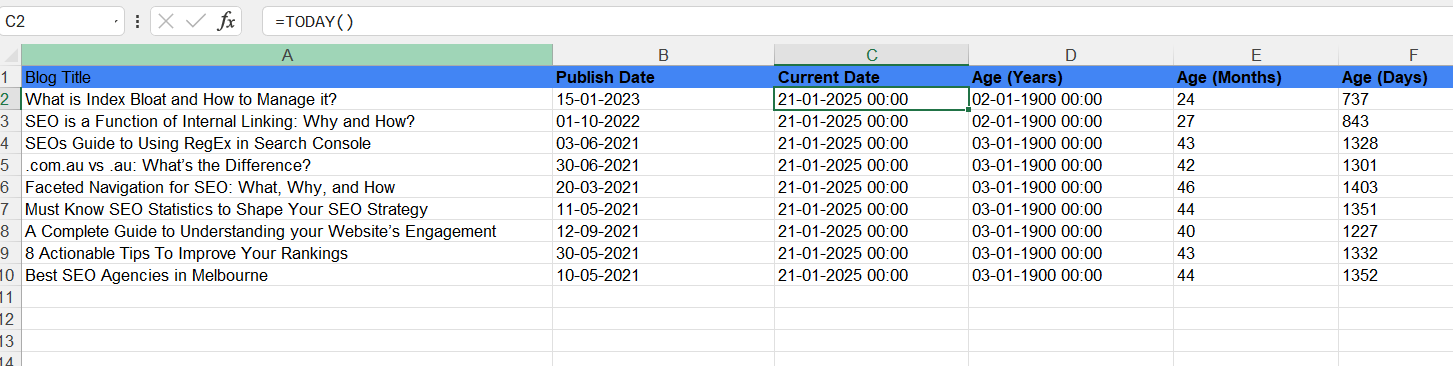
Image Note: One arrow should point at the formula, and another drag-down arrow should point at the “current date” in cell C2.

Next, we enter =DATEDIF(B2, C2, “Y”) in column D to calculate the age in years. It shows the number of full years between the publish date in column B and today’s date. We drag the formula down, as shown in the screenshot.

Image Note: One arrow should point at the formula, and another drag-down arrow should point at cell D2.

In column E, we use =DATEDIF(B2, C2, “M”) to calculate the age in months. It shows the total number of months that have passed. Again, we drag the formula down to apply it to all rows, as shown in the screenshot.

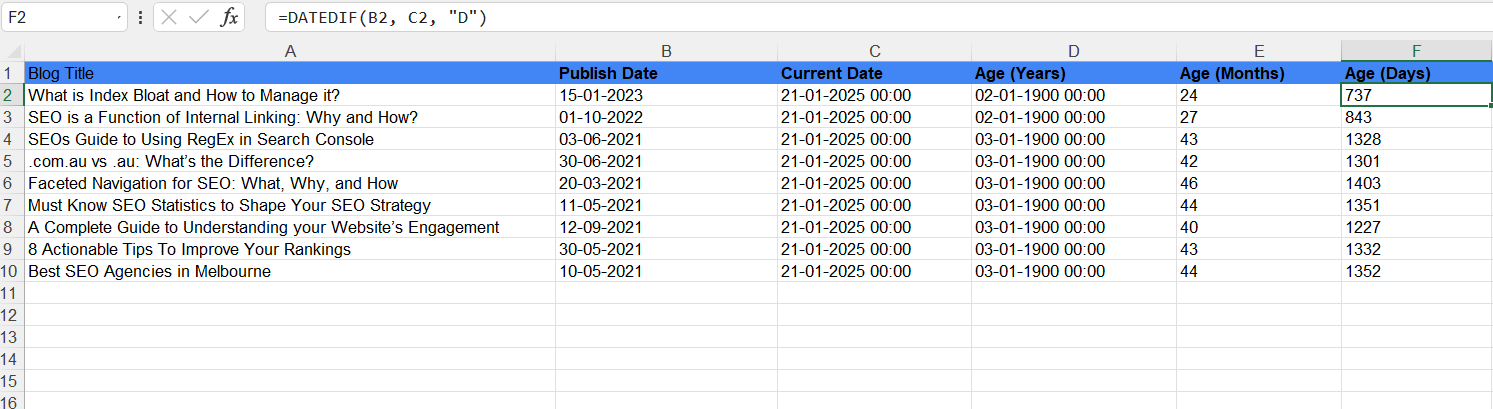
Image Note: One arrow should point at the formula, and another drag-down arrow should point at “737” in cell F2.

TEXT

TEXT function allows you to convert a number to text in a specific number format, making it useful for formatting dates, times, numbers, and other data in a readable format.

Syntax: TEXT(value, format_text)

SEO use cases:

Formatting dates for consistency in reports
Converting numbers or percentages into a more readable format for reports or summaries.
Ensuring uniformity in how data appears, like formatting dates as “dd/mm/yyyy” or turning large numbers into a more readable form (1,000,000 as “1M”).

Example:

Let’s say we want to format dates in the “Blog Publish Date” column to display in a more readable format, like “Month Day, Year” (like this - “January 15, 2023”).

So, here, we will use the TEXT function to format the date: =TEXT(A2, “mmmm dd, yyyy”).

The output will display the date in a more user-friendly format - “January 15, 2023,” as shared in the screenshot below. Drag down the formula to see similar output for all the dates.

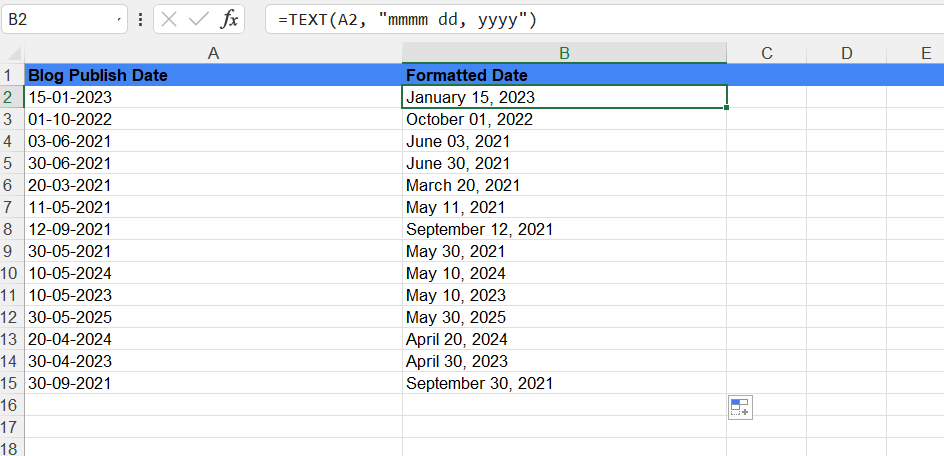
Image Note: One arrow should point at the formula, and another drag-down arrow should point at “January 15, 2023” in cell B2.

8. STATISTICAL FUNCTIONS

Statistical functions in Excel allow you to analyse data by calculating key metrics like averages, medians, and frequency distributions. These functions are crucial to finding insights from large datasets.

AVERAGE

The AVERAGE function helps you calculate the average numeric value of the data for selected cells.

Syntax: AVERAGE(number1, [number2], …)

SEO use cases:

Counting average search volume of related keywords
Calculating average keyword difficulty for a group of matching keywords
Calculating the average traffic generated by a group of matching keywords, etc.

Example:

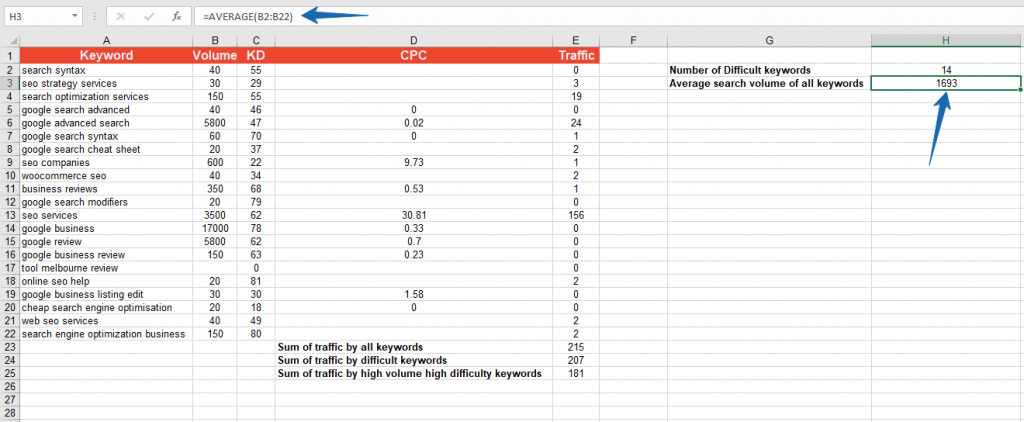
We have the search volumes in Column B and we want to calculate the average search volume for this set of keywords. We applied the formula =AVERAGE(B2:B22) in cell H3.

As you can see, it returned the average value in H3.

As you can see, it returned the average value in H3. You can use this function to get the average search volume and difficulty while considering whether to target a group of keywords as a part of your content and SEO strategy.

MEDIAN

The MEDIAN function allows you to calculate the middle value of a given set of numbers or the average of the two middle values when there is an even number of data points.

Syntax: =MEDIAN(number1, [number2], ...)

SEO use cases:

Calculating the median daily traffic to understand a page’s performance unaffected by extreme spikes or dips in traffic.
Finding the median ranking position of a website across multiple search engines.
Identifying the median character count of meta descriptions or title tags.

Example:

Let’s say we want to analyse the median daily traffic to pages on a website over the past week. The median identifies the middle value and offers a better analysis than average traffic.

So, we collect daily traffic data for your pages over seven days and arrange it in rows.

Now, we can calculate the median daily traffic for the first page (row 2) using the formula =MEDIAN(A2:H2).

Dragging the formula down to apply it to all rows will help calculate the median traffic for each page.

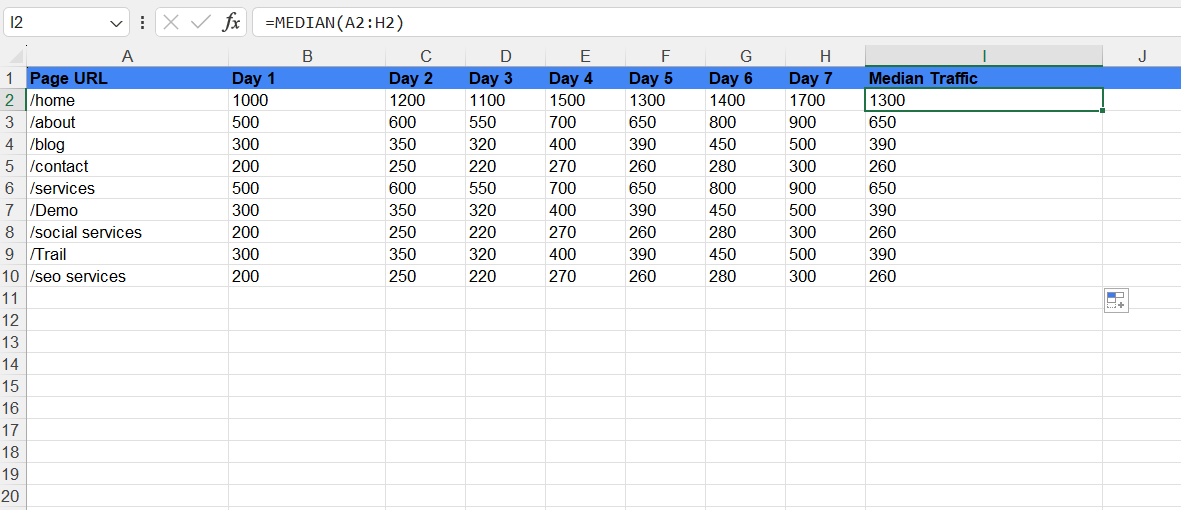
Image Note: One arrow at the formula and dragging down the design arrow at 1300.

STDEV

The STDEV function allows you to calculate the standard deviation of a set of values, which measures how spread out the numbers are from the average. This can help determine the variability in data.

Syntax: =STDEV(number1, [number2], ...)

SEO use cases:

Understanding fluctuations in traffic data or click-through rates (CTRs).
Analysing the spread of rankings for a particular website or page.

Example:

Say we compile daily traffic data for our website pages over seven days and arrange it in rows.

Now, we need to use the formula =STDEV(A2:H2) to calculate the standard deviation of traffic for the first page (row 2).

Dragging the formula will give traffic variability for each page, as shown in the screenshot below.

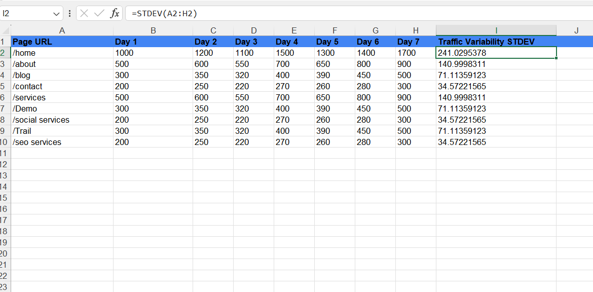
Image Note: We need to show one arrow at the formula and one drag-down arrow at 241.0295378

PERCENTILE

This function returns the Kth percentile of a range of values, which reflects the value below which a given percentage of observations fall.

Syntax: =PERCENTILE(array, k)

SEO use cases:

Identifying the 90th percentile for each page’s daily traffic can help find top-performing days.
Leveraging data to decide which pages could benefit from optimisation during peak traffic.

Example:

Let’s say we want to calculate the 90th percentile of traffic for different pages on our website (to analyse top-performing pages).

So, we collect daily traffic data for the past week and arrange it in rows.

Now, we use the formula =PERCENTILE(A2:H2, 0.90) to calculate the 90th percentile for the first page (row 2).

Dragging the formula will help us calculate the 90th percentile for each page, as shown in the screenshot below.

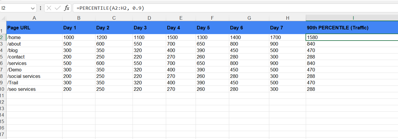
Image Note: We need to show one arrow at the formula and one drag-down arrow at 1580.

9. CONCATENATION AND SPLITTING

Concatenation allows you to combine text from multiple cells into a single string. It can be used to create URLs, metadata, or custom formats in Excel. On the other hand, splitting allows you to divide text in a cell into multiple parts based on a delimiter. It helps organise and analyse data.

CONCATENATE

The CONCATENATE formula allows you to combine data from two or more cells into one.

Syntax: CONCATENATE(text1, [text2], …)

SEO use cases:

Creating a final URL from the text in different columns with data such as website names, categories, slugs, etc.
Merging the first and the last names from different columns — Useful for link-building outreach Bulk keyword research, etc.

Example:

We have the website name, category, and slug in different columns — A, B, and C — and we want to create the final URL by merging them.

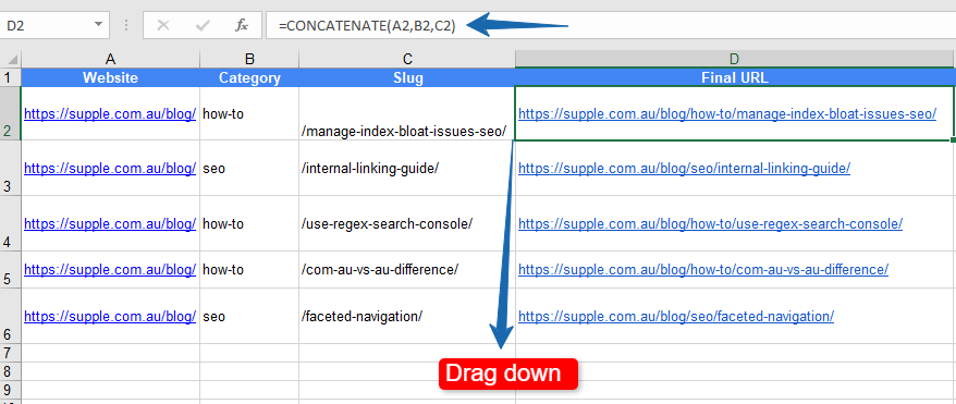
So we entered the formula =CONCATENATE(A2,B2,C2) in cell D2 and we got the final URL. Next, we dragged down from cell D2 to D6 and we got the entire list ready.

Thus, this formula can come in quite handy when you want to create URLs at scale.

TEXTJOIN

This function allows you to combine text from multiple cells into one cell, separating each value with a specified delimiter. This can help to combine text data such as URLs, addresses, or names from various cells.

Syntax: =TEXTJOIN(delimiter, ignore_empty, text1, [text2], ...)

SEO use cases:

Combining domain, path, and query parameters to form a complete URL.
Concatenating keywords, brand names, and product descriptions for SEO content
Creating meta tags (title, description) by combining data from different cells for optimisation.

Example:

We have a list of product categories, IDs, or filters in separate cells. Now, we want to generate a URL for each product.

We will use the formula =TEXTJOIN(“”, TRUE, A2, B2, C2) to build URLs for SEO. It combines the Domain (A2), Path (B2), and Query Parameter (C2) to generate a full URL.

Dragging down the formula will give results for all the domains, as shown in the screenshot below.

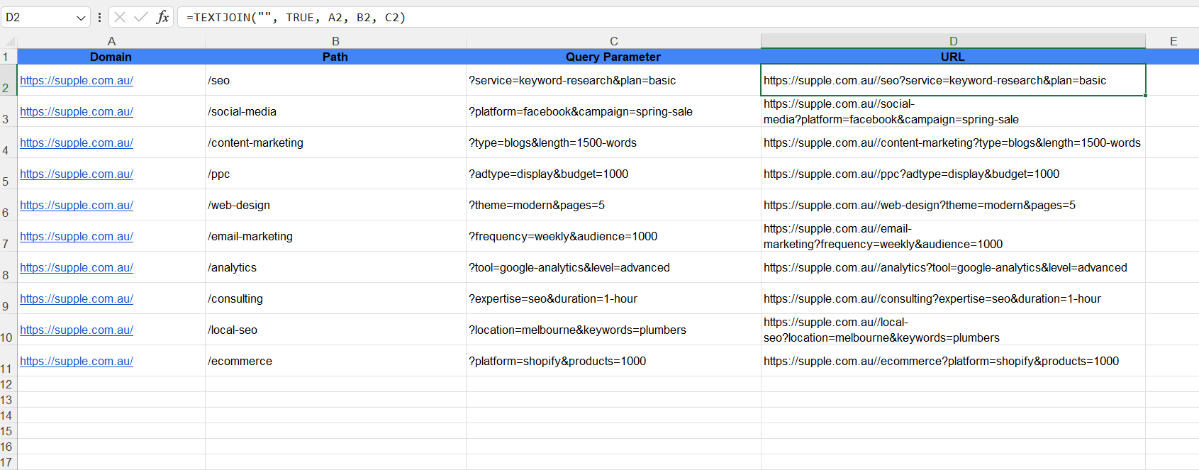
Image Note: We need to show one arrow at the formula and one drag-down arrow at the URL in D2.

SPLIT (in Google Sheets)

The SPLIT function in Google Sheets helps divide the contents of a single cell into multiple cells based on a specified delimiter. This allows you to break a string into individual components, such as separating first and last names or splitting a URL into its components.

Syntax: =SPLIT(text, delimiter, [split_by_each], [remove_empty])

SEO Use Cases:

Separating keywords when you have a cell containing multiple keywords separated by commas.
Breaking down a URL into its domain, path, and query parameters.
Splitting meta titles and descriptions.

Example:

We have a dataset of keywords separated by commas. Now, we use the SPLIT function in Google Sheets to split multiple keywords into separate cells across a row. We use the formula: =SPLIT(A2, “, “).

Dragging the formula down will automatically split the keywords in all the rows, as shown in the screenshot below.

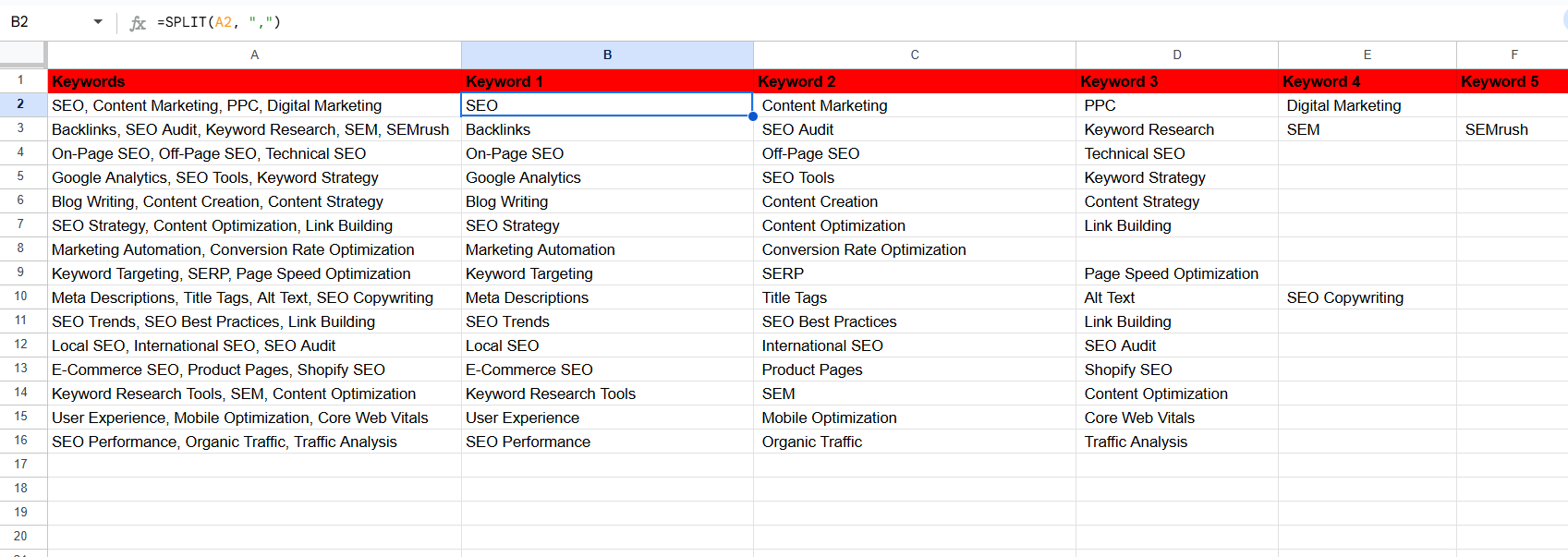
Image Note: We should show one arrow at the formula and one drag-down arrow at B2.

10. ADVANCED FORMULAS

We will discuss advanced formulas in Google Sheets that can help you perform complex data analysis, automation, and decision-making.

QUERY (Google Sheets)

This function allows you to retrieve and analyse data based on specified criteria, similar to SQL queries. It can filter, sort, and aggregate data based on conditions you define.

Syntax: =QUERY(data, query, [headers])

SEO use cases:

Filtering product keywords that contain a specific term.
Sorting keyword data by search volume, relevance, or other metric.
Aggregating keyword data by count, sum, or average (useful for metrics like clicks or impressions).

Example:

Suppose we have a dataset in cells A1:D6 with data like keywords, search volume, clicks, and impressions. We want to extract only the rows with the keyword “SEO” and sort these results by search volume in descending order.

For example, keywords like “SEO tips” and “Local SEO checklist” could be part of this dataset.

Now, we will apply the formula in cell E: =QUERY(A1:D6, “SELECT A, B WHERE A CONTAINS ‘SEO’ ORDER BY B DESC”, 1)

This formula extracts only the keywords with “SEO” from column A and their corresponding search volumes from column B. It then sorts the results in descending order of search volume.

For instance, “Local SEO checklist” (1800 search volume), “SEO strategies” (2000), and “SEO tips” (1500) appear in the filtered results, sorted by search volume.

Notice how the output looks in the screenshot below.

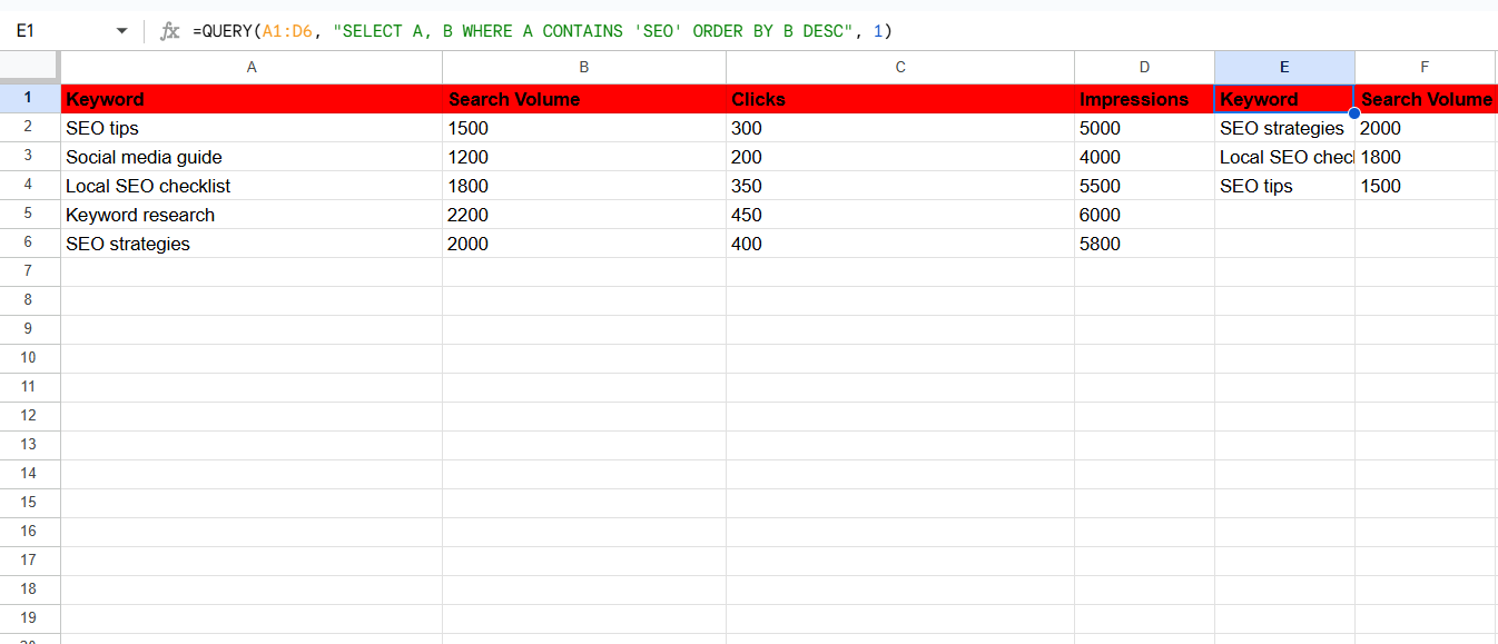
Image Note: One arrow at the formula and one at the KEYWORD table on the right side.

GETPIVOTDATA

This function allows you to extract specific data from a pivot table by referring to field names and items.

Syntax: =GETPIVOTDATA(data_source, field, [item1, item2, …])

SEO use case:

Extracting organic traffic metrics like clicks, impressions, or CTR from a pivot table summarising traffic by channel.
Tracking keyword performance by fetching metrics like conversions or bounce rates.
Pulling metrics like mobile traffic or location-specific impressions to break down SEO performance by device or geographic location.

Example:

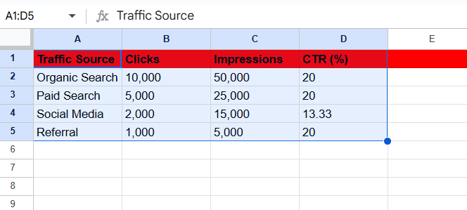
We have a dataset summarising SEO performance metrics like clicks, impressions, and CTR for different traffic sources. See the below shared screenshot.

Now, we create a pivot table to make this data more interactive.

First, we highlight the dataset and go to Insert → Pivot Table, placing it in a new sheet, as shared in the screenshot below.

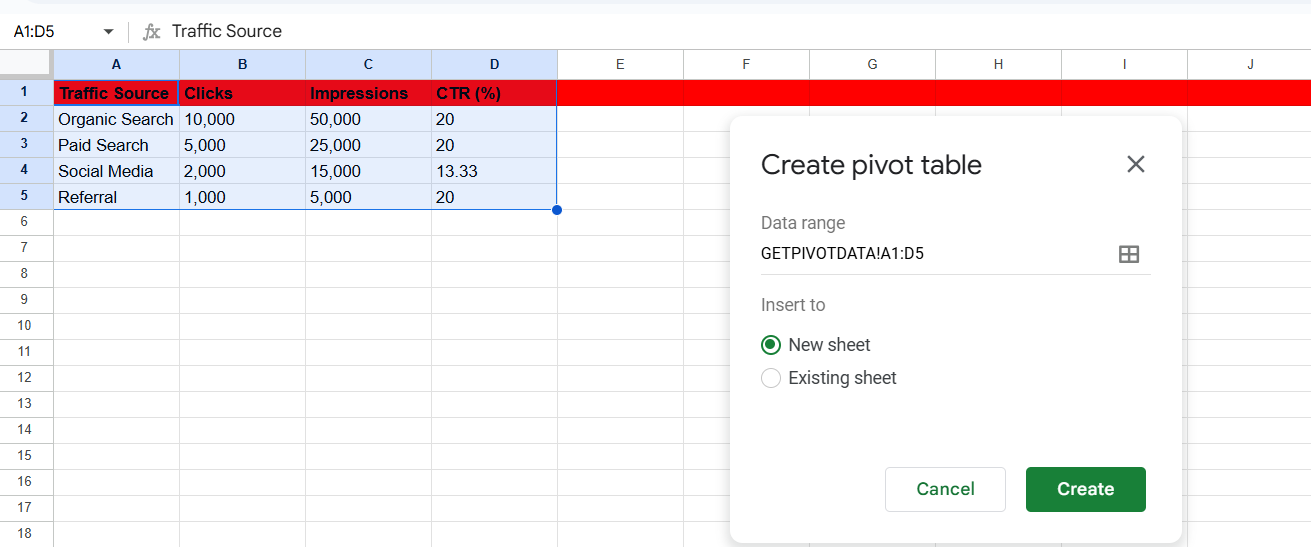
Note: Arrow at pivot table

Next, we add Traffic Sources to rows and include Clicks, Impressions, and CTR (%) as Values in the Pivot Table Editor.

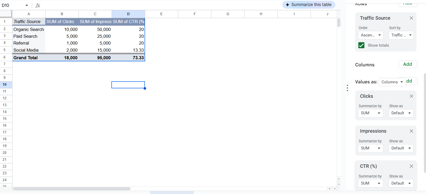
Image Note: Arrow at right side - traffic source, clicks, impressions, CTR.

Next, we want to extract specific data dynamically from this pivot table. For instance, the number of clicks for “Organic Search.” So, we used the Excel formula for SEO and retrieved the value of 10,000, as shared in the screenshot.

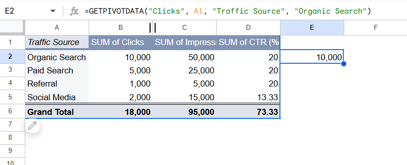
Image Note: One arrow at formula and another at 10,000 - no dragging down here.

Additional Tips for Mastering Excel for SEO

Here are a few crucial additional tips for mastering Excel for SEO.

Combining Formulas

SEO data often involves multiple variables, such as keywords, rankings, traffic, and conversions. Combining formulas can help with in-depth data analysis and create dynamic, automated processes that save time.

For instance, we can combine VLOOKUP and IF to analyse SEO data dynamically.

Here’s how.

Say we have the following dataset (A1:C6).

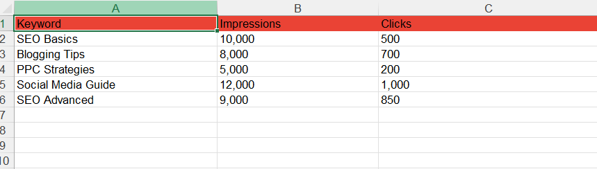
We will use VLOOKUP to find the number of clicks for specific keywords from the dataset. We will combine it with IF to categorise the performance as “High” or “Low” based on a click threshold (for example - 500).

First, we will create a search keyword list and add the keywords to analyse (D2:D4).

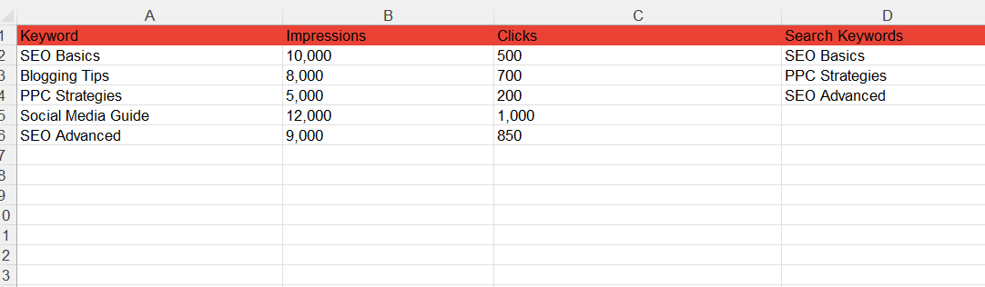
Now, combining VLOOKUP and IF, we will use the formula -

=IF(VLOOKUP(D2, A2:C6, 3, FALSE) > 500, “High”, “Low”)

Here, VLOOKUP(D2, A2:C6, 3, FALSE): Finds the number of clicks for the keyword in D2 from the dataset.

IF(... > 500, “High”, “Low”): Categorises performance as “High” if clicks are more than 500; otherwise, “Low.”

Dragging the formula down will give us the output, as shown in the following screenshot.

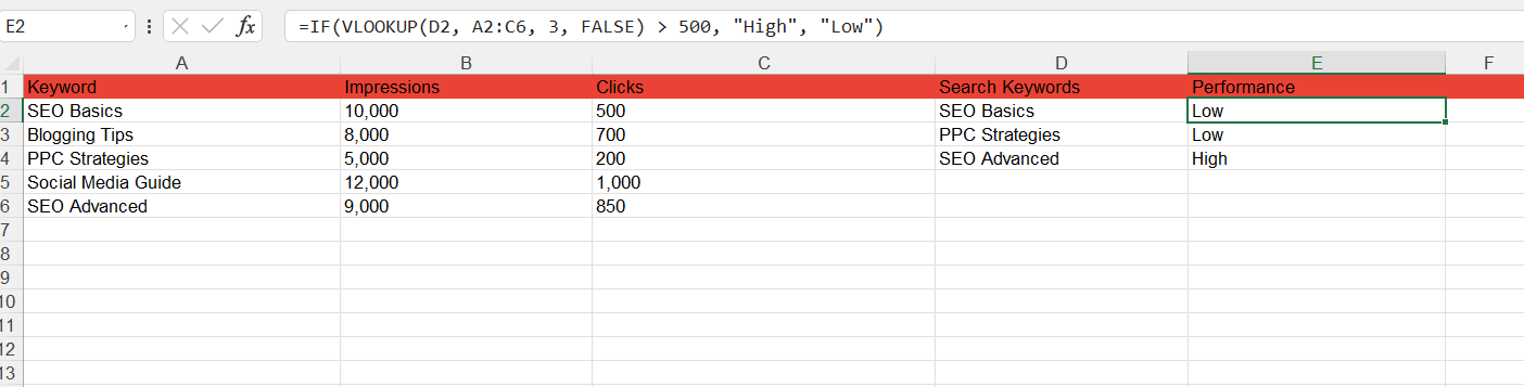
Image Note - One arrow should point at the formula and one at E2: low.

Automation Excel Tools for SEO

Here are a few crucial automation Excel tools for SEO to consider.

1. SeoTools for Excel: This powerful plugin is designed for SEO professionals. It offers advanced tools for on-page, off-page, and backlink analysis.

Source

Its key offerings include:

On-page SEO functions like HtmlH1, HtmlTitle, and HtmlMetaDescription to check page setup.
Off-page SEO functions like CheckBacklink to verify backlinks are still available.
Automated KPI reports with Google Analytics integration.
Backlink profile analysis using Majestic integration.
Custom Connectors via XML format for API integration.
Crawl pages using the Spider tool with a URL list.

2. SEOgadget for Excel: Another excellent tool that allows SEO professionals to connect Excel with Majestic, Moz, and other SEO platforms. This comprehensive add-in tool is designed to enhance SEO workflows directly within Excel. It provides a range of functions for analysing website performance, backlink data, keyword rankings, and more.

Source

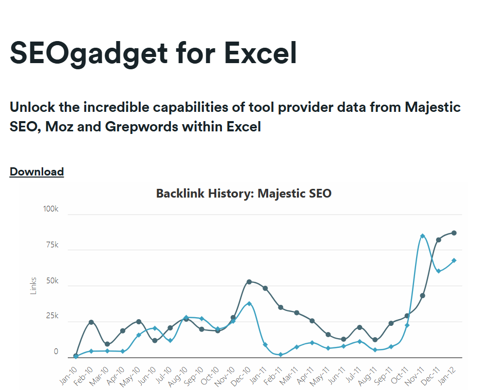
Its key offerings include:

Keyword rank tracking across search engines
Backlink analysis and link quality checks
Search traffic data from Google Analytics.
Detailed SERP analysis for competitive research
Automated and customisable SEO reports in Excel
Google Analytics data access within Excel
Bulk URL analysis for SEO metrics

3. Analysis ToolPak: A built-in Excel add-in that provides advanced statistical analysis capabilities.

Source

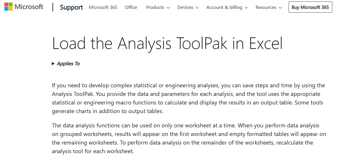
Its key offerings include:

Statistical analysis tools for data insights
Histograms and basic descriptive statistics
Regression analysis
Correlation and covariance matrices

YouTube Channels to Learn Microsoft Excel

Here are a few YouTube channels teaching Excel. They offer step-by-step tutorials to help you master formulas, data analysis, and automation.

ExcelIsFun: This YouTube channel is perfect for beginners and advanced users. The author covers Excel formulas for SEO, data analysis, and creative solutions.
Leila Gharani: This channel offers engaging tutorials on everything from basics to advanced tools like Power Query and VBA.
My Online Training Hub: This channel shares comprehensive Excel for SEO tutorials covering dashboards, reporting, and data visualisation. The author uses easy-to-digest language to keep things simple.
Ignasius Ryan: This channel is a good resource for learning niche tips and tricks. The author uses an easy-to-understand language and focuses on various Excel formulas for SEO and other real-life applications.
Office Tutorials: This channel shares tutorials that can improve your work productivity using Excel formulas for SEO.

Learn Excel for SEO with AI

You can learn Excel for SEO with AI-powered, free-of-cost tools like ChatGPT and Microsoft Copilot. Whether you are a beginner or an advanced user, these platforms provide real-time assistance, simplifying complex formulas and functions. For instance, ChatGPT can guide you through the step-by-step processes of Excel. Besides, you can leverage Copilot to learn the concepts of Excel, troubleshoot issues, and automate SEO tasks.

The best part? You don’t need to pay a single penny and can master Excel for SEO at your own pace.

Wrapping Up

And that’s a wrap.

If the majority of your working time goes into working with large SEO datasets, the above formulas can save you a lot of time.

Initially, it may take some time to understand and practice these formulas. But once you master them, you’ll be much more productive in your daily SEO tasks.

Excel isn’t just a spreadsheet tool. It’s one of the most powerful marketing tools to analyse, visualise, and manage large datasets. Combining these formulas with other SEO marketing tools, like keyword research or analytics platforms, can help you create a data-driven SEO strategy that delivers results.

Besides, if you need a helping hand with your SEO strategy, feel free to reach out to us.

Authors

Hardy Desai

Hardy is the visionary founder of Supple Digital, a boutique SEO agency based in Melbourne, Australia. With a profound understanding of the digital landscape and a deep passion for innovation, Hardy has steered Supple Digital to become a leading name in the SEO domain.